Q-LocalSearch

“This time I won’t make any silly jokes or references”, that’s what SHE said !

In today’s article, I’m gonna try to explain to you what I’ve been doing for the last week, and any comment or suggestion would be great, even if you feel that you are not concerned, maybe you are looking at it from an angle that could help, and you can find the the full code in this link ( make sure to choose the branch : “local-search-rl” ).

Anyway, in this part of the code, you can see that there’s the initial local search function and the q-local search one, it’s good to maintain the extensibility of the code, so when I need to implement a new algorithm, all I have to do is choose between them since they do not affect the other parts.

def bso(self):

i=0

while(i<self.maxIterations):

print("refSol is : ",self.refSolution.solution)

self.tabou.append(self.refSolution)

print("Iteration N° : ",i)

self.searchArea()

print("********************************************************")

print("Search zone is :")

for k in range (self.nbrBees):

print(self.beeList[k].id)

print(self.beeList[k].solution)

print("*******************************************************")

#The local search

for j in range(self.nbrBees):

self.beeList[j].reward = 0

self.beeList[j].localSearch()  # This is the initial local search

self.beeList[j].ql_localSearch()  # This is the q-local search

print( "Fitness of bee " + str(j) + " " + str(self.beeList[j].fitness) )

self.refSolution=self.selectRefSol()

i+=1

If we consider the initial algorithm of local search at the level of a bee, it does an exhaustive search, in other words it takes the solution, flips all its bits 1 by 1, and evaluates each time, which makes the complexity, if we take it as the cost of training a model, equivalent to the number of attributes of the model (for example the sonar dataset, has 60 attributes, this means we would train 60 models ) and this is only for a single bee, and for a single iteration, which makes the complexity : o(Max Iter x Nbr Bees x Nbr Local Iter x Nbr Attributes)

This is the initial local search function :

def localSearch(self):

best=self.fitness

#done=False

lista=[j for j, n in enumerate(self.solution) if n == 1]

indice =lista[0]

for itr in range(self.locIterations):

while(True):

pos=-1

oldFitness=self.fitness

for i in range(len(self.solution)):

if ((len(lista)==1) and (indice==i)and (i < self.data.nb_attribs-1)):

i+=1

self.solution[i]= (self.solution[i] + 1) % 2

quality = self.data.evaluate(self.solution)

if (quality >best):

pos = i

best=quality

self.solution[i]= (self.solution[i]+1) % 2

self.fitness = oldFitness

if (pos != -1):

self.solution[pos]= (self.solution[pos]+1)%2

self.fitness = best

else:

break

for i in range(len(self.solution)):

oldFitness=self.fitness

if ((len(lista)==1) and (indice==i) and (i < self.data.nb_attribs-1)):

i+=1

self.solution[i]= (self.solution[i] + 1) % 2

quality = self.data.evaluate(self.solution)

if (quality<best):

self.solution[i]= (self.solution[i] + 1) % 2

self.fitness = oldFitness

The idea behind Q-LocalSearch is to provide a sub-set of “filtered” data ( which remains optional ), to flip the attributes intelligently, or in other words, according to a policy, to avoid the exhaustive search.

We begin by explaining what is Q-Learning:

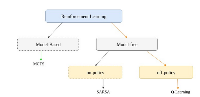
Q-learning is a model-free, off-policy reinforcement learning algorithm proposed by (Watkins & Dayan, 1992). It consists of evaluating the goodness of a state-action pair. Q-value at state s and action a, is defined the expected cumulative reward from taking action a in state s and then following the policy.

Reinforcement learning basic classification

Q-Table

Q-Table is just a fancy name for a simple track-keeping table, like ADL said in his article. It consists generally of a 2D-array, where the rows represent the states and the columns, the possible actions, and because when you deal with feature selection, it’s not wise to use a static data structure, so I am using a list[the index is nbrOnes(state)] of dictionaries[the key is “state”] of dictionaries[the key is “action”] ( a dictionary or dict in python, is like a HashMap in JAVA )

q_table[nbrOnes(state)][“state”][“action”]

Q-function

The Q-learning algorithm is based on the Bellman Optimality Equation given below :

Q(state, action) = R(state, action) + Gamma * Max[Q(next state, all actions)]

The Q-function explained

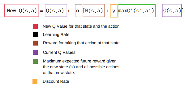
And that’s how we update the table each time, and we use the q-values to pick the next state, which is in this case, what attributes to flip, and here’s the Q-LocalSearch function :

def ql_localSearch(self):

for itr in range(self.locIterations):

state = self.solution

self.fitness = self.data.evaluate(state)

if not self.data.ql.str_sol(state) in self.data.ql.q_table[self.data.ql.nbrUn(state)]:

self.data.ql.q_table[self.data.ql.nbrUn(state)][self.data.ql.str_sol(state)] = {self.data.ql.str_sol(state):{}}

action = self.data.ql.step(self.data,state)

next_state = self.data.ql.get_next_state(state,action)

accur_ns = self.data.evaluate(next_state)

self.data.ql.learn(self.data,state,action,self.fitness,next_state)

self.solution = next_state.copy()

Recap

To recap what we’ve done here today, we talked about Q-learning, and how we used it to make a so called Q-LocalSearch function, which is a way to use Q-learning algorithm for feature selection.

And for this model we have :

• state : is a combinaison of features
• action : flipping a feature
• reward : for now, we consider the accuracy ( fitness ) of the state-action as a reward, but in the next article maybe, we will go deeper and see why it’s not the optimal way to define it.

I really hope you enjoyed it, I’m trying to put everything that I judge important, and if you need more details do not hesitate to leave a comment, or PM me.

And yeah, you can always check my last article.

The "local search" problem - part 2

Last time we talked about the problem of continuously having new data to consider which makes us re-train our model, this time, we will try to see how studies are trying to find a solution by reducing the dimension (X in the last example) of the datasets.

The feature selection for classification can be seen as a combinatorial optimization problem whose objective is to select a subset of n attributes from an initial set of N attributes such as n<N and quality of a solution can be the quality of the classification model constructed using this subset of attributes. The search space contains (2^n) solutions, thus, it is considered as an NP-hard problem, and often approximate methods such as metaheuristics are used to find a good quality solution in a reasonable time.

In a previous work, a metaheuristic based on local search called Bee Swarm Optimization (BSO), was used to solve the feature selection (FS) problem, and to “take you back to when it all first started”

A clue : it’s a song :D

Our project consists of introducing reinforcement learning to this existing method, so first I’m going to briefly present the algorithm, and what could be improved in the local search.

The Bee Swarm Optimization (BSO) metaheuristic is inspired by the foraging behavior of real bees : a bee starts by leaving the hive in order to find a flower and gather nectar. Then, it returns to the hive and unloads the nectar. If the food source is rich, the bee communicates its direction and distance to its mates via a dance. The other bees naturally follow the one that indicates the best food source.

First, an initial solution is generated randomly or via a heuristic. This solution will be the reference solution, refSol, from which a search region, a set of candidate solutions, is determined. After that, each solution is assigned to a bee as a starting point of a local search. At the end of the search, each bee communicates its best found solution to the other ones through a table, named dance.

The problem with the actual definition of best found solution is that we consider a solution as a vector of bits mapped to the actual set of features ( 1 the feature is used , 0 not used ), and the quality of a solution is the classification accuracy returned by the used subset. The problem with that is that we do not consider the effect or contribution of an added/removed feature, and we think that this is a great opportunity to use reinforcement learning methods, and try to find a good policy to keep the most relevant features based on the effect of a subset of features.

If you have any comments, suggestions let me know in the comments, I could really use some help ( in fact, I switched to medium based on a friend’s suggestion, for me it’s all the same )